May 19, 2018 by akhilendra
Data Exploration in R with GGPLOT2 & Standard Functions

In this post, we are going to perform high level data exploration in R programming language using GGPLOT2 and its standard plotting functions. So if you are looking on information on how to make plots and graphs in R using ggplot2 or standard r functions, you will find this post useful. You can simply change the name of the data sets and other parameters to reuse them for your project.
I am not going to add details about data because the purpose is to show few common and important commands.
if you have any question, please leave your question or comment.
Minimum Steps for exploration:
- Importing the data set into R
- Understanding the structure of data set
- Graphical exploration
- Descriptive statistics
- Insights from the data set
Data Exploration in R
please make sure you set the working directory correctly so that R can find your file. please note i have included the output for reference but you will need to print it in your machine to understand it better.
I have used GGPLOT2 and standard R functions for plotting. if you want to use GGPLOT2, you will first need to install the package.
#Importing the data set into R

library(rJava)

library(xlsxjars)

library(xlsx)

lung= read.xlsx("LungCap_Dataset.xls", sheetIndex = 1, header = TRUE)
lung
Output
library(rJava)
> library(xlsxjars)
> library(xlsx)
> lung= read.xlsx("LungCap_Dataset.xls", sheetIndex = 1, header = TRUE)
> lung
LungCap.cc. Age..years. Height.inches. Smoke Gender Caesarean
1 6.475 6 62.1 no male no
2 10.125 18 74.7 yes female no
3 9.550 16 69.7 no female yes
4 11.125 14 71.0 no male no
5 4.800 5 56.9 no male no
6 6.225 11 58.7 no female no
7 4.950 8 63.3 no male yes
8 7.325 11 70.4 no male no
9 8.875 15 70.5 no male no
10 6.800 11 59.2 no male no
11 11.500 19 76.4 no male yes
12 10.925 17 71.7 no male no
13 6.525 12 57.5 no male no
14 6.000 10 61.1 no female no
15 7.825 10 61.2 no male no
16 9.525 13 63.5 no male yes
17 7.875 15 59.2 no male no
18 5.050 8 56.1 no male no
19 7.025 11 61.2 yes female no
20 9.525 14 70.6 no female no
21 3.975 6 57.3 no male no
22 5.325 8 59.7 no female no
23 10.025 16 72.4 no male no
24 8.725 11 68.0 no male yes
25 9.375 11 65.7 no female no
26 8.350 12 61.3 no male yes
27 6.750 12 60.7 no female no
28 9.025 9 65.6 no male no
29 1.125 4 48.7 no female no
30 10.475 18 72.0 yes female no
31 4.650 4 53.7 no female no
32 7.725 13 64.7 no male no
33 10.600 13 69.3 no male no
34 11.025 13 65.6 no male yes
35 8.650 12 67.8 no male no
36 8.825 10 65.5 no male no
37 4.200 6 52.7 no male no
38 8.775 9 63.6 no male no
39 6.325 11 64.6 no female no
40 11.325 17 77.7 no male no
41 8.225 14 65.4 no female no
42 10.725 17 72.5 no female yes
43 5.875 8 58.9 no female no
44 7.275 12 67.7 no male no
45 1.575 6 49.3 no male no
46 6.700 11 62.6 no female no
47 7.650 11 61.7 no male yes
48 8.000 12 64.7 no female no
49 12.950 17 74.9 no male no
50 7.350 7 61.6 no male no
51 9.625 15 66.4 no male no
52 12.425 15 74.1 no male no
53 7.400 11 65.3 no male no
54 4.875 10 61.4 no male no
55 12.225 18 79.6 no male no
56 4.250 6 52.9 no male no
57 8.200 13 65.6 no male no
58 11.400 19 79.1 no male no
59 4.625 9 56.8 no female no
60 7.825 12 65.4 no male yes
61 6.700 12 57.9 no female no
62 9.200 14 68.2 no male no
63 6.950 9 61.4 no female no
64 6.850 13 58.7 no female no
65 8.450 13 65.1 no male no
66 7.350 13 67.5 yes female no
67 5.375 11 59.3 yes female no
68 7.375 11 63.0 no female no
69 8.600 11 64.4 no female no
70 7.900 12 68.0 no male no
71 8.500 14 61.4 no female yes
72 9.700 11 72.4 no male no
73 5.125 11 51.5 no female yes
74 7.825 13 71.0 no female no
75 6.250 13 61.8 no female no
76 4.975 12 62.6 yes female yes
77 7.500 14 66.6 no male no
78 5.875 9 59.0 no female no
79 10.050 17 70.4 no female no
80 10.800 11 69.8 no male no
81 7.350 12 63.0 no female no
82 11.900 16 69.3 no male no
83 12.050 17 72.2 no male no
84 11.575 19 78.2 no female no
85 6.200 14 61.1 no female no
86 6.125 12 63.3 no female yes
87 13.875 19 78.4 no male yes
88 7.750 11 63.5 no female no
89 7.475 15 63.0 yes female no
90 11.575 19 75.5 no male no
91 6.950 9 63.9 no male yes
92 9.200 14 69.4 no male no
93 9.750 13 72.8 yes male no
94 9.650 14 65.2 no female no
95 11.750 19 78.0 yes female yes
96 10.825 18 75.7 no female no
97 7.550 16 71.1 yes male no
98 6.950 7 64.7 no male no
99 10.675 16 74.9 no male no
100 6.100 10 57.0 no male no
101 8.025 13 66.2 yes male no
102 9.225 14 66.9 no male no
103 3.450 13 58.5 no female yes
104 10.725 16 75.6 no female no
105 7.950 16 67.3 no female no
106 3.425 5 51.7 no female no
107 10.875 16 75.5 no male no
108 8.625 12 64.8 no male no
109 6.450 7 63.2 no male no
110 3.100 7 52.1 no male no
111 10.425 15 70.6 no male no
112 12.150 18 76.3 no female no
113 1.850 8 49.8 no female no
114 5.875 3 55.9 no male no
115 9.125 15 73.4 no male no
116 8.975 15 67.5 no female yes
117 3.750 7 50.3 no female no
118 10.275 18 71.0 no male no
119 6.675 8 54.9 no female no
120 11.775 17 76.9 yes male no
121 8.550 16 67.9 no male no
122 6.450 12 61.0 yes male yes
123 13.200 17 78.6 no male yes
124 11.550 16 75.7 no male no
125 12.950 19 79.6 no male yes
126 7.825 12 67.5 no female yes
127 10.550 17 71.8 no male yes
128 11.700 19 76.2 no female yes
129 3.650 12 56.6 no male yes
130 6.650 12 60.0 yes female yes
131 10.425 15 67.2 no male no
132 12.925 17 75.7 no female no
133 7.450 13 61.1 no male no
134 8.600 12 60.1 no female no
135 10.650 16 74.4 no male no
136 4.725 13 65.5 no female no
137 7.550 15 69.3 no female no
138 10.175 15 71.4 no female no
139 6.450 14 61.4 no male no
140 9.475 13 67.4 no male no
141 4.975 6 58.4 no male no
142 9.900 18 70.9 no female no
143 10.200 18 68.6 no female no
144 12.400 18 81.8 no male no
145 6.850 9 65.7 no female yes
146 11.825 17 73.9 no female no
147 8.625 14 66.8 no female yes
148 11.350 14 70.5 no male no
149 8.225 14 64.0 no female no
150 0.507 3 51.6 no female yes
151 5.075 11 61.2 no male no
152 6.450 8 62.7 no male no
153 6.725 9 56.1 no male no
154 4.525 8 55.5 no female no
155 9.275 16 67.2 no female no
156 2.850 7 51.4 no female no
157 9.350 11 71.2 yes male no
158 5.550 5 55.8 no female yes
159 10.350 16 73.5 no male yes
160 6.625 11 62.4 no male yes
161 9.725 16 68.6 no female yes
162 4.900 10 56.8 no female no
163 10.475 12 69.7 no male no
164 10.850 19 70.9 no male no
165 5.150 7 58.4 no female no
166 4.425 8 56.6 no male no
[ reached getOption("max.print") -- omitted 559 rows ]
Summarizing Data in R for exploration
let’s summarize data and go through some of the most common parameters.
# summaries data to understand it further

summary(lung)

#use str to understand the structure of dataframe

str(lung)

# use table to get the frequency

table(lung$Age..years.)

# get mean & standard deviation

mean(lung$Age..years.)
sd(lung$Age..years.)
Output
> summary(lung)
LungCap.cc. Age..years. Height.inches. Smoke Gender Caesarean
Min. : 0.507 Min. : 3.00 Min. :45.30 no :648 female:358 no :561
1st Qu.: 6.150 1st Qu.: 9.00 1st Qu.:59.90 yes: 77 male :367 yes:164
Median : 8.000 Median :13.00 Median :65.40
Mean : 7.863 Mean :12.33 Mean :64.84
3rd Qu.: 9.800 3rd Qu.:15.00 3rd Qu.:70.30
Max. :14.675 Max. :19.00 Max. :81.80
> str(lung)
'data.frame': 725 obs. of 6 variables:
$ LungCap.cc. : num 6.47 10.12 9.55 11.12 4.8 ...
$ Age..years. : num 6 18 16 14 5 11 8 11 15 11 ...
$ Height.inches.: num 62.1 74.7 69.7 71 56.9 58.7 63.3 70.4 70.5 59.2 ...
$ Smoke : Factor w/ 2 levels "no","yes": 1 2 1 1 1 1 1 1 1 1 ...
$ Gender : Factor w/ 2 levels "female","male": 2 1 1 2 2 1 2 2 2 2 ...
$ Caesarean : Factor w/ 2 levels "no","yes": 1 1 2 1 1 1 2 1 1 1 ...
> table(lung$Age..years.)

3 4 5 6 7 8 9 10 11 12 13 14 15 16 17 18 19
13 6 20 25 37 41 40 51 58 68 69 56 64 54 43 43 37
> mean(lung$Age..years.)
[1] 12.3269
> sd(lung$Age..years.)
[1] 4.00475
Random sampling
sample(lung)
random sampling with size
sample(lung, 5)
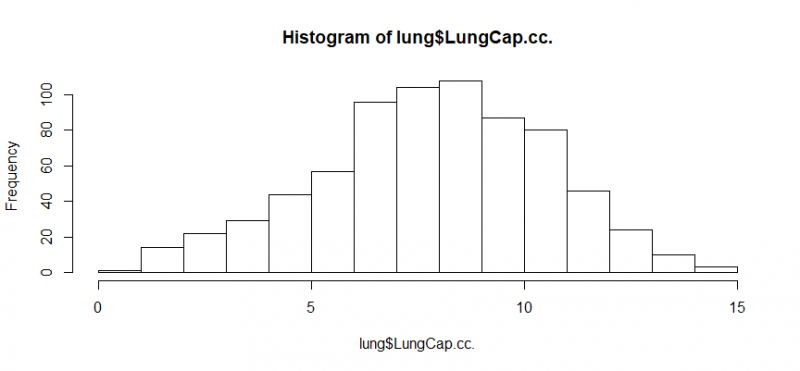
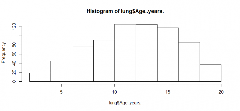
Create histograms in R with standard hist function
hist(lung$LungCap.cc.)
hist(lung$Age..years.)
stem(lung$LungCap.cc.,scale = 1,width = 80,atom = 1e-08)
 0 | 5
   1 | 012356678999
   2 | 00033345666777778999999
   3 | 0011222344445667777788999999
   4 | 001122233333344445555556666677777788899999
   5 | 00000001111122222223333334444455566666677777778899999999
   6 | 00000111111111111122222222222223333334445555555555555566666666667777+13
   7 | 00000000001111112222233333333333344444444444444555555556666666666677+20
   8 | 00000000000000001111111122222222333333333444444444444445555555556666+32
   9 | 00000000000011111111122222222223333333444445555555555666666667777777+11
  10 | 00000000111111112222222333333444444444555555555566666667777777777788
  11 | 0000001111111222222333344455556666677777888889999
  12 | 01111222223333444456799
  13 | 000111234449
  14 | 467
stem(lung$Height.inches.,scale = 1,width = 80,atom = 1e-08)
 The decimal point is at the |

  44 | 3
  46 | 604478
  48 | 01278902389
  50 | 357000124556777999
  52 | 001777888990223567778899
  54 | 2357899901111244555566666677899
  56 | 001112334556666667788889901123334445789
  58 | 000334444455555677778889990012222223333444457777889999
  60 | 0000111222233444445566677789001111122233444444555566667788889999
  62 | 00001111112344455666666778888990000122233333334444445555566667779999
  64 | 00011111233444455667777778889990000111123333344444444555555566666677
  66 | 00000011122233333444445555666678899990112223333444455555556666777778
  68 | 00001111222223334444566666677788889990000111222333333344444466777788
  70 | 0011222344445555668899999000011112222233444455556667788899999
  72 | 00012223444455555667889900111233344555555566667788999
  74 | 000012222334456677899901223445556677778889
  76 | 012233456688992467
  78 | 024469913668
  80 | 388
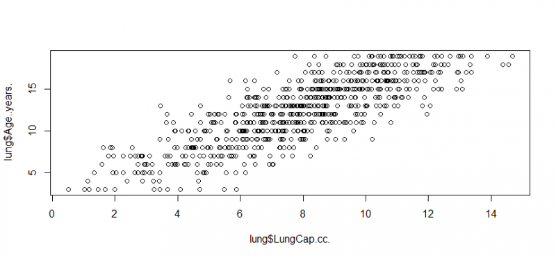
Plot Functions in R
plot(lung$LungCap.cc.,lung$Age..years.)
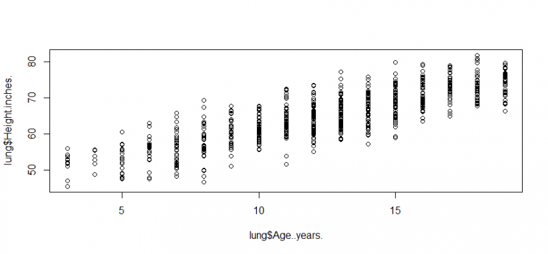
plot(lung$Age..years.,lung$Height.inches.)
Plotting with GGPLOT2
if you need details about ggplot2 library, please visit my previous post on it. Click Here.
now let’s use ggplot2
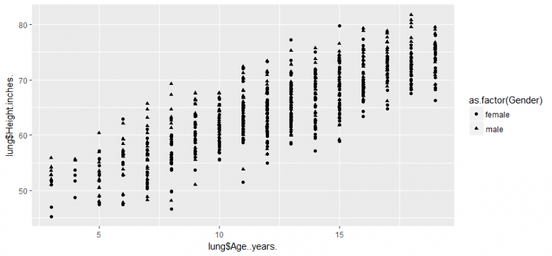
library(ggplot2)
# age..years & lung$Height.inches. are x & y axis here
# i have used shape to group them based on gender

qplot(lung$Age..years.,lung$Height.inches.,data = lung,shape=as.factor(Gender))
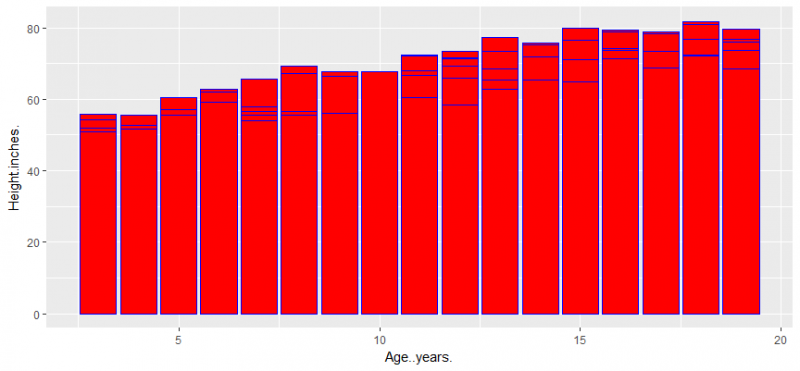
let’s create a bar chart and add color by using fill and colour
ggplot(data = lung, aes(x=Age..years., y=Height.inches.)) + geom_bar(stat = "identity",position = "dodge",colour= "blue", fill = "red")
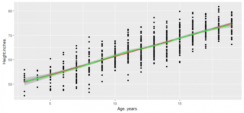
now create a scattered plot with ggplot2 with a fitted line
sctplot<-ggplot(data = lung, aes(x=Age..years., y=Height.inches.)) + geom_point()

sctplot<- sctplot + geom_smooth(method ="lm", col="red")

sctplot + geom_smooth(col="green")
let’s also add boxplot in the mix
boxplot(lung,las=1)
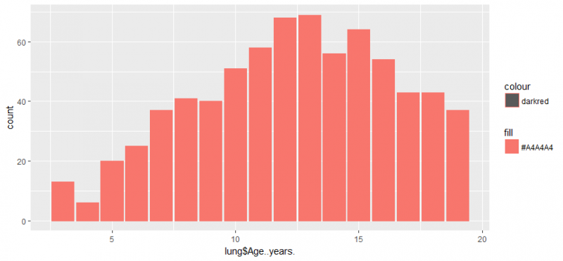
Let’s create more charts using already used commands in this post:
g <- ggplot(lung, aes(lung$Age..years.))
g + geom_bar()
g + geom_bar(aes(weight = lung$Age..years.))
g + geom_bar(aes(fill = '#A4A4A4',, color="darkred"))
As mentioned earlier, objective of this post is to show some of these useful R and ggplot2 commands. If you are looking for something specific, please share your question, i will try to answer that.
Leave a Reply