May 4, 2021 by akhilendra
Gradient descent optimizers- Stochastic gradient descent- RMSprop-Adam-Adagrad
Gen AI & Prompt Engineering program
Unlock the full potential of AI with prompt engineering! Discover how tailored prompts can solve your toughest challenges—faster, smarter, and more efficiently. Start mastering the art of prompting today
If you are working on deep learning model like convolutional neural network (CNN), you must have come across this line in your code.
[Yourmodel] in the above line is presenting your model.
Now most deep learning enthusiasts or students have questions on loss, optimizer, and metrics.
In this post, we are going to address optimizer.
But before we start with optimizers in deep learning, you need to understand that training a deep learning model is an iterative process. You run your model on data set multiple times, this is called epoch.
Your model will product an output of continuous numbers or classes/labels for regression and classification respectively.
To put simply, each iteration is intended to reduce or minimize the loss function.
What is optimizer
Needed to improve learning of a deep learning model.
Update weight and bias in back propagation based on error.
May slow down the model if dealing with large dataset.
So, let us understand what is happening here.
As you probably know, we pass bias and weight along with input through neural network and model produces an output.
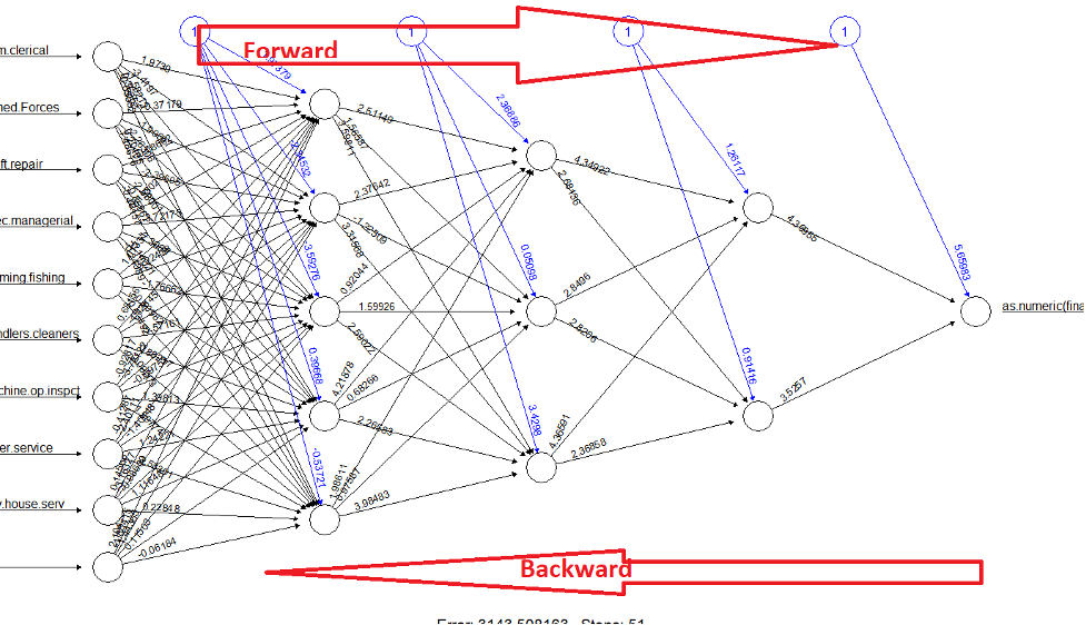
Step 1- model performs forward propagation, produces an output and loss is calculated.
Step 2- model performs back propagation and based on loss (residual error), bias and weights are adjusted to reduce the error.

Please refer to post on evaluation metrics for details on residual errors. Click here.

So as mentioned earlier, you need an optimizer to reduce the error. There are many optimizers which can be used in deep learning, but we are going to focus on some of the most popular optimizer algorithms.
Please note in machine learning objective is to NOT over train model because that will result in overfitting. So, you are not essentially looking to achieve 0 error. You are essentially training your model in an optimum range.
Some of the algorithms which we will cover in this post are.
Gradient descent
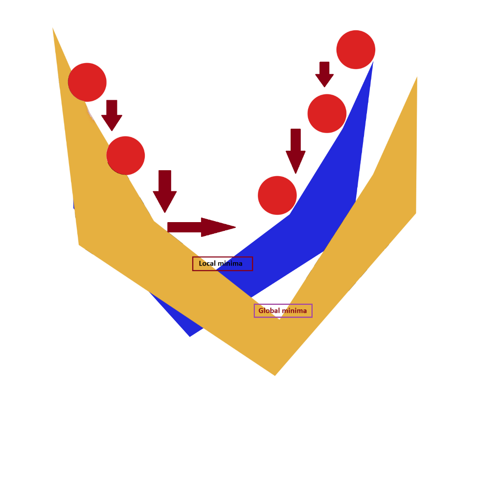
Now if you look at this image, red circle represents weight. And difference between global minima and value of red circle is error.

Objective here is to reach global minima which is 0.
But remember as mentioned earlier, it is 0 theoretically. In deep learning or machine learning, we are essentially looking to reduce this error. We are not interested in 0 because it could result in overfitting but still theoretically, it should be 0.
Therefore, idea is to reduce it. Now look at this table for MAE for illustration.
Actual Value (y) | Predicted Value (y hat) | Error (difference) | Absolute Error | |
100 | 130 | -30 | 30 | |
150 | 170 | -20 | 20 | |
200 | 220 | -20 | 20 | |
250 | 260 | -10 | 10 | |
300 | 325 | -25 | 25 | |
21 | Mean | |||
Note- You take the absolute value of error which is the positive value, therefore -30 becomes 30 | ||||
Click here to learn more about MAE and other evaluation metrics.
Primary objective of gradient descent or any other optimizer is to reduce this error.
During back propagation, weights are adjusted, and output is recalculated. And as shown in the figure, it is a step-by-step process where gradually model will try to adjust the weight and reduce the error.
But sometime, it reaches a local minimum and get stuck.
Also, please note that though I have used arrows which are showing downward movement, it will be zigzag followed by lots of oscillation.
One of the biggest challenges in developing any deep neural network model is to control the descent or this movement while applying optimizers or performing gradient descent.
Now look at this clip, as you can see it is constantly changing and moving randomly. There is no fixed direction. Therefore, it is a very hard to control this movement.
We apply two additional parameters along with optimizers while optimizing a model. These two parameters are.
- Momentum
- Learning rate
Please note momentum and learning rate are used with all optimizers and not just gradient descent.
One of the biggest disadvantages of gradient descent is that it works on entire dataset which means if there are lot of data points in your dataset like a million or more, it could take ages to update all the weights.
In current world where most machine learning or deep learning probably deals with extremely large dataset, gradient descent is simply not feasible.
You need lot of time and resources if you plan to use it. Therefore, other optimizers are most common. But before we continue with them, let’s spend some time on momentum and learning rate so that it will be easier for you to understand other optimizers used in machine learning or deep learning.
Momentum in simple terms is acceleration or speed which you are passing as an argument with your optimizer to ensure that descent does not get stuck at local minima and should have enough momentum to pass through it. It is usually passed along with optimizer as an argument and it should be greater than 0. If you do not specify Keras will default it to 0.
But do not go overboard with it, it is usually considered as bad idea to have a very high momentum. Something under 1 is fine. You should play with it and tweak it multiple times to validate the performance of your model.
Learning rate
Learning rate in deep learning is another important hyperparameter which is usually between 0 to 1 and it is used for scheduling the learning of your model.
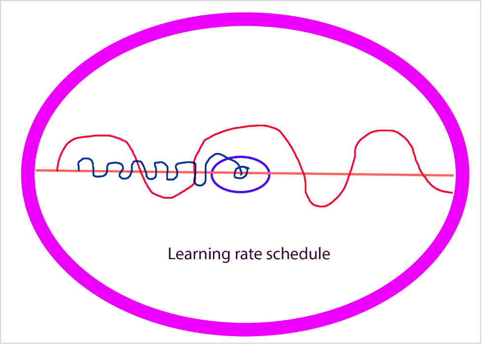
You can think of learning rate schedule as a step. With this hyperparameter, you are essentially controlling the size of the step which model should take while minimizing the loss function or optimizing the weights.
So, it is the value by which model should update the weights in back propagation to minimize the loss.
You need to randomly set a value between 0 to 1 while compiling your model. If you do not specify, most packages will default it to 0.
For example, if you, as a person, takes larger step, you could probably jump over the center but if your step size is too small, you will need more steps to reach that point.

It works similarly.
If you’re learning rate is too small, it will take lots of steps to arrive at the convergence whereas if your step is too large, you could miss it entirely.
So, if you refer to MAE table shown earlier in this article, you will see that the difference in the first row is 30 (absolute error). Now if your model is trying to reduce this error and your learning rate is too small, your model will need too many steps to reach that point which means gradient descent will be too slow or worst-case scenario, gradient descent may get stuck at local minima and never reach that point.
And if learning rate is too large, gradient descent could just overstep it and cross it.
So, one of the biggest challenges with learning rate is identifying the appropriate value for it.
Problem as mentioned earlier is simple, if you are learning rate is too small, your model could take forever to train and if it is too large, it could simply miss it.
To counter this problem, there are variations of learning rate where objective is to counter the side effects of a constant learning rate.
You can specify the learning rate schedule to vary based on epoch. This is also referred as decaying learning rate.
Keras offer 4 types of learning rate schedules/decay algorithms.
- Exponential Decay
- Piecewise Constant Decay
- Polynomial Decay
- Inverse Time Decay
You can click on following link if you need to learn more about these- https://keras.io/api/optimizers/learning_rate_schedules/
But in a nutshell, you should reduce the learning rate as the training progresses. So idea is to use a higher learning rate for initial epochs and then apply some kind of function or formula (like the ones mentioned above) to reduce the learning rate.
These perform better than fixed learning rate.
lr_schedule = keras.optimizers.schedules.ExponentialDecay(
initial_learning_rate=1e-2,
decay_steps=10000,
decay_rate=0.9)
optimizer = keras.optimizers.SGD(learning_rate=lr_schedule)
Source link- https://keras.io/api/optimizers/
In the above-mentioned code, we are applying exponential decay and specifying decay rate. Similarly, you can specify other variations of learning rates also.
This is popular and useful while compiling your deep learning models like CNN etc.
Please note all the algorithms mentioned in this post are gradient descent-based optimizers which means they use gradient descent to minimize the loss.
There are few other techniques also, but they are not covered here.

Stochastic gradient descent
Stochastic gradient descent is a variation of gradient descent. By default, instead of using all the data points from a dataset, you are randomly selecting 1 data element and updating its weight.
So, you can imagine that it will be so much faster.
Therefore, it is a much popular optimizer in deep learning. It is also known as SGD.
There is another version of SGD where instead of 1, you are taking a mini batch out of entire dataset and using that.
But by and large, its core benefit is that it helps in speeding up the training. But sometimes it causes huge fluctuations in loss so watch for that.
Adagrad
Adagrad or Adaptive Gradient descent Optimizer is all about dynamically updating the learning rate. Gradient descent by itself, will apply same learning rates to all the weight across all the layers and across all the epochs.
With Adagrad, you do not need to manually control the learning rate.
It will adapt to features. for example, while working on parameters associated with frequent features, it will apply smaller learning rate whereas while working on less frequent features, it could apply larger learning rate.
In fact, because of this feature it has gained lot of popularity in recent past. But by design, learning rate will drastically fall which leads to very little to No learning after few epochs. This happens because in adagrad’s formula, sum of squared gradient descent will continue to accumulate in denominator which results in a big denominator over time which essentially means that learning rate will become very small.
RMSprop
RMSprop counters adagrad’s problem of increasing denominator by using the decaying average of squared gradient which essentially means it will account for recent gradient descent more than the distant ones. This helps in controlling the denominator.
By and large it is like adagrad except this one difference due to which there is no sharp fall in learning rate. It helps in ensuring that your gradient does not overshoot near minima.
It is also an adaptive learning rate which means it uses different learning rate for different parameters.
Adam
Adam (Adaptive Moment Estimation) is one more method that computes adaptive learning rates for each parameter.
Adam is essentially a hybrid of adagrad and RMSprop or you can say it takes best of both. So Adam starts with adagrap followed by RMSprop and finally weight optimization.
This way, it stores an exponentially 5 decaying average of past squared gradients, but it also keeps an exponentially decaying average of past gradients. What it means is that it gives more weightage to recent momentum than the earlier ones.
If you remember, the challenge with adagrad was that it kept accumulating squared gradients which resulted in higher denominator which led to low learning rates. With this ADAM, this issue is resolved.
It is one of the best optimizers as it is easy to implement and work on most problems.
Don't forget to share it with your friends & families to help them too.
Leave your comment if you have any feedback or question.

Leave a Reply